---

A LiDAR Simulation

LiDAR (Light Detection And Ranging) is finally becoming an affordable replacement for the IR and ultrasonic ranging sensors typically used on hobby robots. This article uses a simulation to experiment with some unique ways of using LiDAR data for simple navigation.

The first installment of this series examined reasons why LiDAR could soon replace the ultrasonic and infrared ranging sensors that have typically been used for navigation on many hobby robots. It was also suggested that a LiDAR simulation could be used to allow experimentation with LiDAR principles without having to purchase hardware. This article will not only discuss such a simulation, it will also use it to explore a totally different way of utilizing LiDAR data for basic navigation.

An Alternative to SLAM

Normally, as discussed in the first article, LiDAR-based systems generally use SLAM software (Simultaneous Localization And Mapping). The internal operation of SLAM is very complicated, and it could be argued that it provides far more capability than many robots need. Imagine a system that simply allows your robot to determine the size and position of various objects around it. This could possibly allow the robot to navigate in a known environment by simply moving toward recognized objects along its path.

This approach is similar to how you might move through your home at night. You might not be able to see clearly, but you should be able to identify large shapes such as sofas, doorways, chests, etc. If you wanted to move to a certain destination from a known position, you might move toward a large chair that you know should be a little to your left. When you get to the chair, you expect to see a doorway a little to your right. You face the doorway and move through it and look for a sofa expected to be slightly left of forward. After moving toward the sofa ... well, you get the idea.

If you know where objects generally are in your environment, you could identify them even in a dimly lit room based on their size and location. And, after moving to one object, you could identify and move to the next, generating a reasonable path to your destination.

Simulating the LiDAR

The code fragment in Figure 1 uses RobotBASIC’s simulated robot to create an array of distances measured at intervals of one degree. It will be assumed that the global variable ScanWidth is the total number of readings to make. The simulated robot turns to the right at an angle equal to half of the total scan. A loop then turns the robot through the scan range to take the distance readings using the rRange() function.

FIGURE 1.

---

At the end of the scan, the robot turns back to its original heading. Most LiDAR systems scan 360°. That is more than we need. So, in this example, the robot only scans the 180° area directly in front of the robot.

At each scan position, there are three pieces of data deposited in the two-dimensional array P. The first index of this array determines which scan data we are accessing. At each of these positions in the array, there are three pieces of data. The information associated with scan number 8, for example, would be stored in P[8,0], P[8,1], and P[8,2]. These three items are the distance measured, a true/false indicator of a discontinuity (more on this shortly), and the angle of this measurement.

In this example, since measurements are made in one degree increments, the angles stored are the same as the index for each measurement. This simply means that the value of P[n,2] will always be n for this program. When we move our discussions of a simulated LiDAR to the real thing, this may not always be true, so designing this option into the program will help ensure future compatibility.

Discontinuities

Once the distance and angular data have been stored in the array P, we need to analyze the information to determine where discontinuities exist in the distance readings. Look at Figure 2.

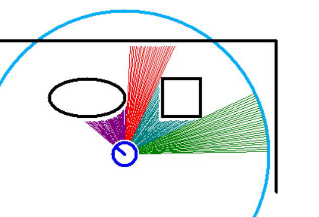
FIGURE 2.

---

It shows a robot with two objects in the corner of a room. When taking the readings, the robot was originally facing towards the right wall and then turned (in one degree increments) counterclockwise.

At each angular position, the robot made a (simulated) distance reading. The length of the lines extending out from the robot indicate the distance measured at that position; the blue arc represents the maximum distance that can be measured for this example. Notice the first group of measurements (green) are all the same length because there’s nothing in the way, so each measurement is the maximum possible.

When the robot turns about 30 degrees, the measurements are obstructed by the corner of the square obstacle. Notice that this causes a large change in the distance measured when compared to the previous measurement. We’ll call this large change a discontinuity.

As the robot continues to turn, the distance calculated decreases with each measurement until the robot is facing the corner of the square object. Notice also that even though the measurements are changing, each new measurement is very close to the previous one, so they will not be considered a discontinuity (in this example, the change in distance must be greater than 10 pixels to be considered a discontinuity).

If the robot continues to turn past the corner of the square object, the measurements will start to increase in small amounts. When the turn is sufficient to make the measurement miss the square object, the reading will change by a large amount, making it another discontinuity.

As the robot continues to turn, the readings are measuring the distance to the upper wall. This continues until the oval object is seen, representing another discontinuity. Notice that the colors of distance measurements change at each discontinuity. Also notice that each color represents a different object. Object is used here as a general term because the seemingly open spaces could easily just be objects (like walls) that are further away.

Object Characteristics

Once we know where all the discontinuities are, it’s easy to calculate how many objects are seen, the angle to the center of each object, and the distance to each object (this will be the shortest distance measured to each object). Figure 3 shows an output from a sample program that performs these calculations and displays the results.

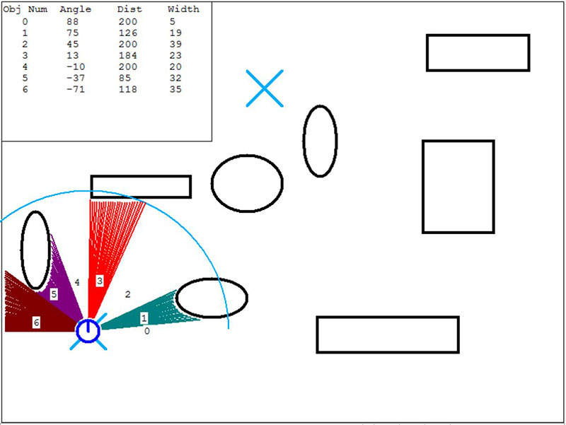
FIGURE 3.

---

Navigational Decisions

The goal of this program is to use the data from the simulated LiDAR to move the robot from the X where it’s currently located to the X in the upper center of the screen. Before each movement, the robot performs a LiDAR scan as shown in the figure.

Notice that the distance measurement vectors for each object are in different colors.

Notice also that if the distance measured exceeds the allowed range for the LiDAR that the vectors are not shown. These open spaces are still considered objects, but leaving those areas white seems to make the information easier to digest.

Each scan area has an object number associated with it.

The upper left corner of the figure shows a table that displays the information calculated for each object. The information in this table is actually stored in the program in a two-dimensional array called OBJ. The first index accesses a particular object and the second determines the information to be accessed (angle, distance, and width).

Choosing the Direction to Move

Looking at Figure 3, it probably makes the most sense for the robot to move forward through the white area labeled 2. Notice from the table that this object is 45° to the right of the robot, 200 pixels away from the robot, and is 39° wide.

It’s very important to realize that if the robot was in a slightly different orientation, this information could be different. For example, if the robot was originally facing slightly to the right of its current orientation, then the small white area labeled 0 might not have been seen at all.

This would mean that the oval object currently called 1 would actually be object 0, which means we would want to move in the direction of object 1 (instead of 2 as shown in the figure). The important point here is that a robot in this general situation should not always move toward object 2. Instead, we need a module that allows the robot to find a large (wide) object that should be forward and right of the robot.

Having such a module could allow the robot to find the direction we want it to move, even if the scan data is not exactly as shown in the figure (because the robot’s position and orientation will seldom be exactly what we expect).

A routine that allows us to find this object is shown in Figure 4.

FIGURE 4.

---

We can call this routine using a statement like this:

call FindObject(ScanCCW,30,Angle)

The first parameter passed tells the routine to perform the search in either a clockwise or counterclockwise direction. During my testing, having this option made it much easier to find the right object (more on this shortly).

The second argument indicates the minimum object width we’re looking for. Since we know the object we want (in this case) is generally going to have a width of around 39 (and the other objects that might be seen first in the search have much smaller widths), we can search for an object at least 30 wide and be assured the proper one will be found.

Another nice thing about the routine in Figure 4 is that it returns in the third parameter the angle to the object from the robot’s perspective. This means the robot simply has to turn that amount and it will be facing in the proper direction for its next move.

We can move the robot forward some predetermined fixed amount and know within a reasonable approximation where the robot will be.

The Second Move

Figure 5 shows the robot after it has moved through area 2 and performed another scan. In this case, we can search CCW for an object of at least width 30 again.

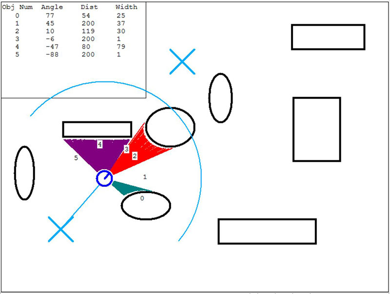
FIGURE 5.

---

This is a good example of why we need to be able to search both CW and CCW. If we had performed this search in a CW direction, it would have found object 4.

To the Destination and Back

We can continue moving the robot and experiment at each position to determine how to find the proper object to move toward as well as the distances to move. Figure 6 shows the robot’s path as it moved all the way to the destination and halfway back to the starting position.

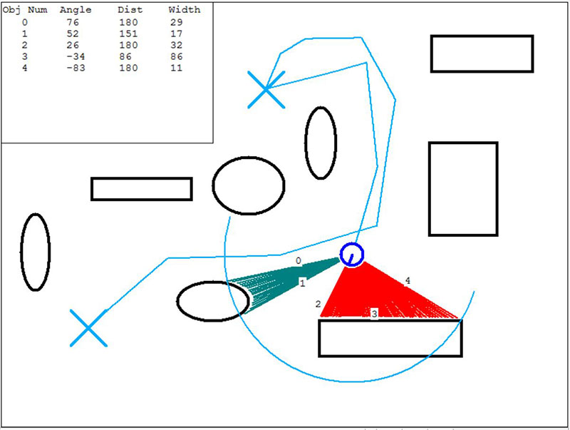
FIGURE 6.

---

Adding Realism

You might think that the experimental values chosen for this path would only work for this particular situation. This is not the case. Look at Figure 7. It shows numerous runs of the round trip made by the robot. What’s interesting about this example is that every movement of the robot had a 2% error. Furthermore, each time the program is run, the position and/or size of the objects are altered slightly.

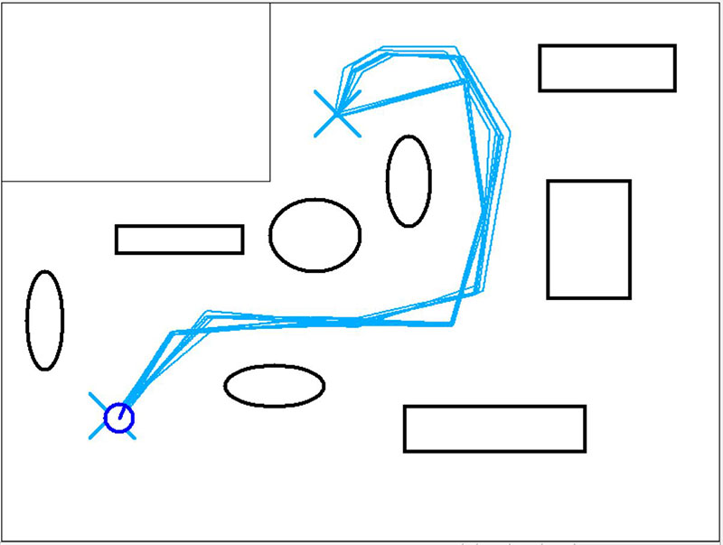
FIGURE 7.

---

What this shows is that the navigational algorithm demonstrated here — even as simple as it is — has the potential to handle basic point-to-point movements in a known environment. Note: In this run of the program, the variable DisplayScan was set to FALSE so that the scan vectors and object details are not shown.

Adding Options

Let me start by admitting that it took a bit of experimenting to determine what objects to look for and how far to move at each position. A major reason for the difficulty is that the only real choice I had was to pick an object to move toward. Things would have been much easier if there were more options available. Let’s look at some examples.

Perhaps the easiest improvement would be to have the option to move the robot forward, not a fixed amount as in this example, but to move until the robot is a specified distance from the destination object. This alone can add greatly to the consistency of the paths traveled in Figure 7 — and they are fairly consistent already. If we’re willing to do a little more work, we can add ways to choose the object that controls the robot’s direction.

Perhaps we could build a better FindObject module that lets the robot look — not only for an object with a minimum width — but perhaps one that is also at least a specified distance away. Or, maybe one that’s less than the specified distance.

Imagine having another module that lets you look for an inside corner (like the corner of a room) or an outside corner (like the front corner of a dresser).

Maybe it could be valuable to build a module that could calculate the angle of the face of an object (relative to the robot itself), so that the robot could align itself either parallel with that object or perpendicular to it. All these options are relatively easy to program and they can make it easier to create a very precise path for your robot to follow.

Experimentation Required

Of course, even if you implement all these ideas, you still have to experimentally determine the series of actions the robot must follow to get from one point to another (from the kitchen to the living room, from the living room to the kitchen, from the living room to the bedroom, etc.). Once you have the details worked out for each path though, you can have the robot choose which set of instructions to follow based on where it is and where it wants to go.

There are certainly many things to consider. Some environments could work well with this approach while others might need SLAM. If you think this approach has merit, or even if you just find it interesting, I encourage you to experiment with some of the ideas discussed in this article. If you use the RobotBASIC simulation discussed herein, you can experiment without purchasing any hardware. RobotBASIC, as well as the source code for the program discussed in this article, can be downloaded free from RobotBASIC.org.

For those readers that want to experiment with this approach using real LiDAR hardware, the next installment in this series will explore some of the problems they might encounter as well as potential solutions.  SV

---