---

Many SERVO readers would love to give their robot the ability to determine its location in a known environment. There are many possible solutions (LIDAR or external transponders, for example), but most options are too expensive for the average hobbyist. This article explores a unique approach with interesting possibilities.

One of the more interesting aspects of hobby robotics — at least for me — is trying to find new and unique solutions to common problems. One such problem is giving your robot the ability to identify its location in a room or home, or even in an artificial environment created for a classroom or computer club demonstration. Over the years, I’ve explored many ideas related to this subject and most have been at least moderately successful in an experimental real world environment.

Recently, I came up with an idea that is software intensive and thus inexpensive to implement. Let me say up front, that I have not developed a turn-key system, but have created working models (both real and simulation) that provide proof of concept. My goal for this article is to present the basic theory in a way that encourages others to experiment with and expand on my work. To that end, the system will be developed using RobotBASIC‘s simulated robot.

Using a RobotBASIC simulation makes it possible for anyone to explore various aspects of the system (RobotBASIC is a free language available from www.RobotBASIC.org). Furthermore, the test program uses variables for controlling many aspects of the algorithm so that users can quickly evaluate different options with minimal effort.

The program is also modularized to make it easy to implement the algorithm with other languages and/or microcontrollers.

The Basic Principle

Ideally, the system should be able to create a repeatable scanning signature for various grids within a room. To find its current location, the robot should perform a scan and compare that signature to a list of stored signatures to find the closest match, thus determining its position in the room.

You could create grids covering the entire room, but for many navigation-oriented projects, it can be more efficient to create multiple groups of grids at various waypoints throughout the robot’s environment. Let’s look at an example.

Figure 1 shows a test environment for our simulation.

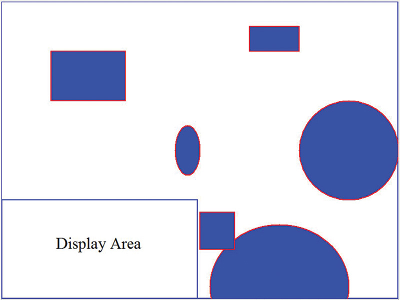
FIGURE 1.

---

The rectangles and circles represent furniture and other obstacles in the room. Notice the Display Area in the lower-left corner. It will be used to display signature information during testing. Figure 2 shows the same environment with five groups of grids.

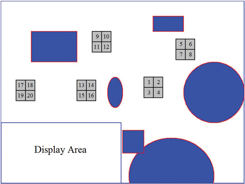
FIGURE 2.

---

Imagine the robot moving from one grid group to another and then using its local positioning system to affirm its current location.

This constant affirmation will prevent the accumulation of position error over time, allowing the robot to constantly correct and adjust to its environment. Of course, the grid size, location, and numbers will be determined by your particular needs and situation.

Creating a Signature

For purposes of this project, the system will scan around the robot’s perimeter using an ultrasonic ranger. It will create a unique number or pattern that can be associated with a general location in the room, and something close to that pattern should be generated as long as the robot is anywhere within the designated area (for example, one of the grids or grid groups shown in Figure 2).

You might assume we’ll just store the ranging data obtained, but this could be many unique values (making comparisons to known signatures difficult); even small changes in the robot’s position would alter this information. What we need is a way to condense the ranging data into an easy-to-compare format and one that will not change dramatically with relatively small changes in the robot’s position.

In order to get the same signature for a variety of positions within a reasonable area, we must avoid creating codes based on absolute distances because all readings will change with the robot’s position. One way to solve this problem is to create a code for each scan distance that is relative to the most previous scan reading.

For example, instead of saying a particular reading is 32 inches, we might say it is higher (or lower) than the previous reading (in the scan). We can further qualify this indicator by specifying if the new reading represents a large or small change from the previous reading. This process can create codes that are more abstract — codes that do not alter dramatically with small changes in the robot’s position.

Code Details

To keep things simple, the signatures used for this project are composed of seven codes (the letter S, and upper- and lower-case versions of L, H, and V). S will be used to indicate that there is very little change from one scan reading to the next (think of S as standing for the Same reading). Notice that two readings (based on two robot positions) do not have to be exactly the same to create the S code. As long as the distances measured are similar, an S will be generated.

If the new scan distance is higher than the last reading, an H code will be used. An L will be the indicator for lower readings. If the change from one reading to the next is moderate, a lower-case version of H or L will be used and upper-case letters will indicate a significant change. If the change from one reading to the next is very large, a V will be used as the indicator. A capital V means there was a very large increase and a lower case v implies a very large decrease. This normalizing of the data can create codes that don’t change substantially as long as the robot is near its targeted location.

Forming and Comparing Signatures

The signature will be composed of a sequence of one letter codes (as described above) for each scan. If, for example, the robot rotates 360° (starting from a north heading) and takes a reading every 30°, there will be a total of 12 readings, making the signature a string of 12 characters.

Because of the normalization, the signatures of relatively nearby positions should not change dramatically, but signatures of totally different locations should be significantly different. We can compare two signatures by simply comparing the individual letters in the strings and counting the number that are the same. The more letters that compare, the more likely the robot’s position has been found.

Testing and Algorithm

Figure 3 shows a path the simulated robot traveled through the environment. Notice it moved to three different locations and moved around slightly at each one. A 36-character signature was created for each position (scan angle of 10°) and printed in the display area mentioned earlier. A number is also shown that indicates how many of the letters matched when the signature obtained was compared to another.

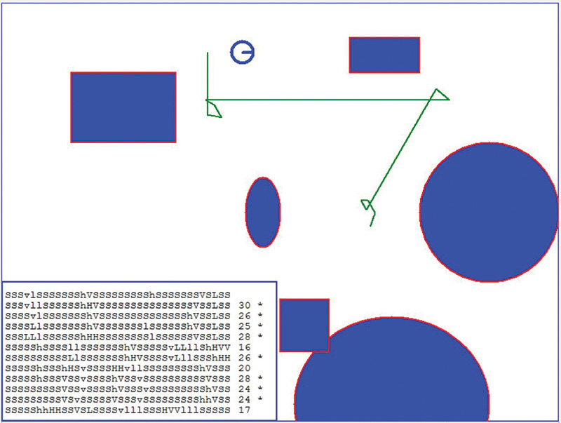
FIGURE 3.

---

An asterisk (*) indicates that the comparison is being made to a nearby location. No asterisk means the comparison is to a remote position and should not be expected to match. Figure 4 shows the signature display area enlarged for improved readability.

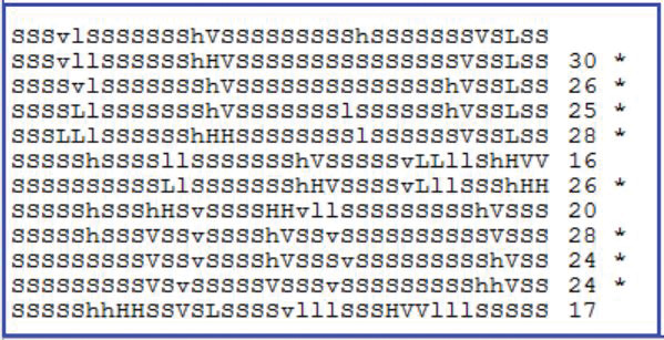
FIGURE 4.

---

The maximum number of correct code matches is 36. As you can see from Figure 4, when the robot is relatively close to its starting position, the number of matches is high; at least 24 in this example, averaging 26.4. When remote locations are compared, their signatures are lower, with scores of 20 or less, averaging 17.7.

Using a Real Robot

A simulated robot provides an easy way to test the ideas presented here, but we need a real world example to verify the validity of the simulation. I used a modified Parallax Scribbler S3 (see Figure 5) with PING))) ranging capability (as discussed in the March 2018 issue of SERVO) to perform some real world scans, although you could use any hobby robot with ranging capability. The S3 currently doesn’t have a compass, so the robot was physically placed at a variety of positions in a make-shift environment.

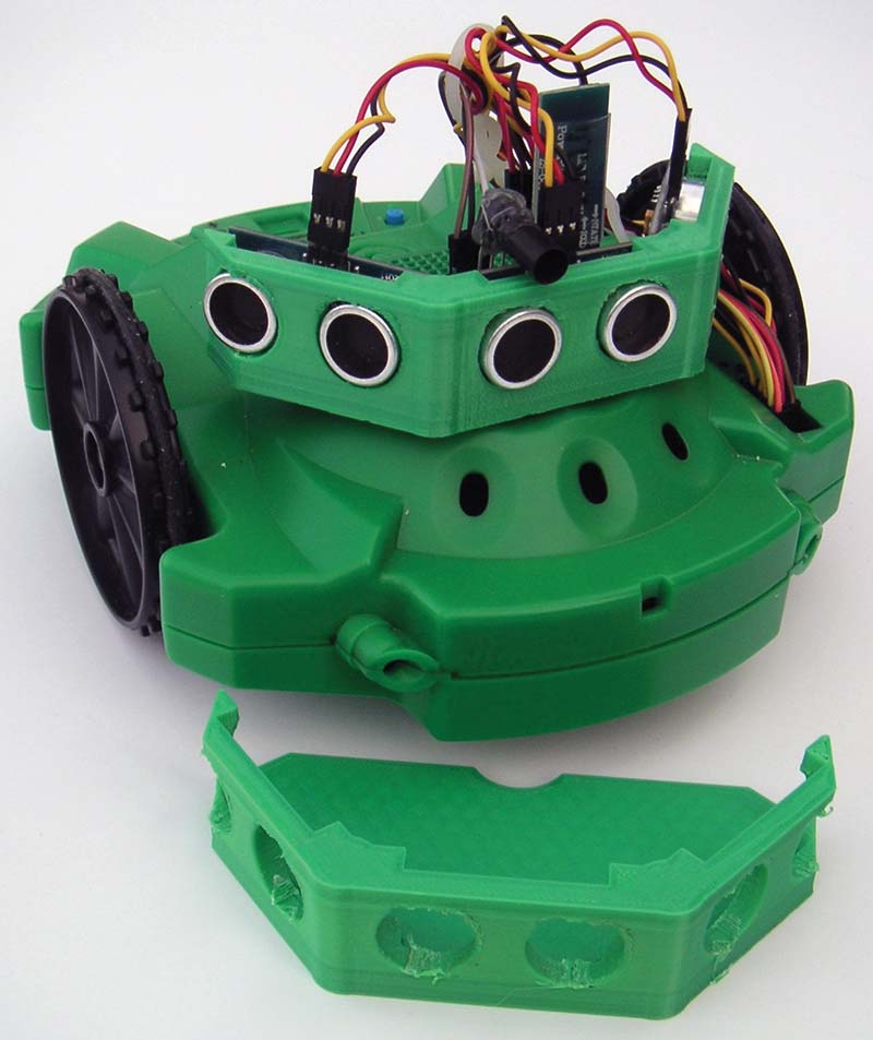
FIGURE 5.

---

Figure 6 shows the results of five scans with the S3. Again, the asterisks show where the signatures should match. For these readings, the robot was moved from its original location a distance approximately equal to its diameter. In all three cases, the readings were very high (27, 26, and 23). When the robot was moved a significant distance (about 40 inches in this case), the signature comparison dropped to 13. Notice that these readings are very similar to that obtained during simulation, verifying its validity.

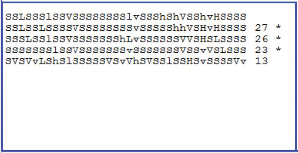
FIGURE 6.

---

One of the reasons the results from the simulation and the real robot agree so well is that care was taken to ensure the simulation properly mimicked the scanning properties of the S3. This is especially important because RobotBASIC’s simulated robot performs a ranging scan in a very narrow beam (like a laser). The PING))) rangers, on the other hand, have a wide beam width.

To provide compatibility, a special routine was written (see Figure 7) that allows the user to specify the simulator’s beam width by passing the left and right angles (a1 and a2).

FIGURE 7.

---

Improving Performance with Experimentation

In my tests, the range comparisons were considered the same if new readings were within 15% of the previous reading. Values differing between 15% and 30% were considered moderate, and those between 30% and 50% were considered significant. Anything larger is considered a very large change, as discussed earlier. All of these parameters are controlled by variables that can be easily changed for experimentation as shown in Figure 8.

FIGURE 8.

---

The code fragment in Figure 9 shows how the signature is formed from the algorithm discussed earlier.

FIGURE 9.

---

The routine in Figure 10 shows how easy it is to compare two signatures. Readers wanting a copy of the entire program can get it with the article downloads or from the In The News tab at www.RobotBASIC.org.

FIGURE 10.

---

Obviously, the algorithm discussed here has potential, but it certainly needs more work to become a complete system. The simulation makes such experimentation easy, quick, and inexpensive.

Keep in mind that in the real world, many factors — such as the robot’s environment and the type of ranging sensor used — could affect the system’s performance. Even so, if your next project requires a local positioning system, you might give this a try.  SV

---